Building Your First Data Pipeline in Google Cloud Platform and dummy data: A Beginner's Guide
Have you ever wondered how does it feel like to work as a Data Engineer and create your own pipeline - from zero to hero (or, in other words, a beatiful dashboard)? Well, I’ve got you covered. Together we will generate dummy data, upload the data to Google Cloud, convert it into a table and output to stakeholders as a dashboard.
The steps will be:
Generate dummy data -> Load to Google Cloud Storage -> Load to Big Query Staging -> Load to Production using Dataform -> Create Looker report
Full code can be found on my GitHub.
Before we begin, you’d need:
Google Cloud Platform project - to create it, please follow the guidelines here
Google Storage Bucket - follow the steps from this tutorial
Cloud Composer instance - to create it, please follow the steps from here. You can keep the default settings for your dummy data project and keep it as small.
Also consider creating a budget cap so that you don’t run into unnecessary costs
Let us begin!
Step 1: Generate dummy data - script #1
Ever felt bored by the publicly available datasets? Well, now you can create your own data. For this project, I will generate a dummy data for a fictional Call Center. I will use the Python faker library; see the snippet of the code below. You can adjust it to serve your own needs.
from faker import Faker

## Initialize Faker
fake = Faker()

def generate_call_center_data(num_records):
    """Generates fake call center data."""
    data = []
    start_date = datetime(2024, 1, 1)

    for _ in range(num_records):
        rep_id = fake.unique.random_int(min=1, max=99999)
        rep_name = fake.name()
        call_id = fake.unique.random_int(min=1, max=999999)
        client_id = fake.unique.random_int(min=1, max=99999)
        client_region = fake.city()
Once we have the data, we need to:
save it as .csv file,
import it to our data lake, which in this case is Google Storage Bucket.
You can do it two ways: Either first save it locally, and then upload, or save it to memory, and directly to Storage Bucket. Since our pipeline will be running in the cloud and the data is small (35 kb), we will save it directly to GCS. Please see the snippet of the code below:
def upload_csv_to_gcs(data, bucket_name, destination_blob_name):
    """Converts data to pandas DataFrame
    and uploads it as a CSV file to Google Cloud Storage."""

    # Convert data to DataFrame
    df = pd.DataFrame(data)

    # Convert DataFrame to CSV format in memory (no local file)
    csv_buffer = StringIO()
    df.to_csv(csv_buffer, index=False)

    # Initialize Google Cloud Storage client and upload the CSV
    storage_client = storage.Client()
    bucket = storage_client.bucket(bucket_name)
    blob = bucket.blob(destination_blob_name)

    # Upload the CSV data directly to the blob
    blob.upload_from_string(csv_buffer.getvalue(), content_type='text/csv')

    print(f"File uploaded to {destination_blob_name} in bucket {bucket_name}.")
Step 2: Write code to consolidate the data into Staging table - script #2
Now that we have our fake data loaded into Google Storage Bucket, we need to do four things:
Load it into the memory from GCS
Mask it (if it contains PII - I will demonstrate it using the rep_name column from my dataset)
Create the staging table in BQ for it
Combine it so that whenever a new file is created in GCS, it gets appended to the table
You can find all the code on my GitHub here, so feel free to download and play around.
Step 3: Write DAG and deploy it in Cloud Composer
Cloud Composer is data orchestration service which - essentially - reads your Python scripts as a series of tasks it needs to perform. We will now deploy our code there and create a sequential pipeline - this is where the fun begins!
When you open the Composer environment you created, you will see a “Open DAGs folder” navigation section. Click it.

You are now in the folder from which Composer sources your code. Whatever you upload to the DAGs folder will be read as a DAG to run.
Since we want to follow the OOP structure, we will keep our auxiliary functions separately and import them into our DAG directly. Click on “create folder” and create a “scripts” folder. Upload the two files you created - the scripts # 1 and 2 - into that folder.
On your machine, create a new my_pipeline.py file.
The way the DAGs work is that you essentially define the tasks one by one.
Let us first import the functions we need from our plugins folder along with some other features we need:
from airflow import models
from airflow.decorators import task
from airflow.exceptions import AirflowException
from airflow.operators.python_operator import PythonOperator
from airflow.utils.trigger_rule import TriggerRule
from airflow.models import Variable

from plugins.read_file_mask_upload import process_and_load_data
from plugins.generate_call_center_data import generate_and_upload_data
And now we move on to the actual DAG creation:
with models.DAG(
    dag_id="call_center_pipeline",
    start_date=datetime(2024, 10, 15),
    schedule_interval=None,
    catchup=False,
) as dag:
Note I set the schedule_interval to None; this is because I don’t need the pipeline to run daily just yet. For now, it will only be externally triggered. If you want it to run daily, change it to ‘@daily’.
Also, please see the catchup = False parameter; it prevents the scheduler from executing missed tasks for past execution dates, ensuring that only tasks for the current and future dates are run.
We will now define the actual tasks that will make the pipeline:
We will first generate dummy data
Then we will expose it to BigQuery Staging table
From there, we will run Dataform job to productionize the data
An example task looks as below; note the kwargs are parameters passed to your Python function:
 generate_data_task = PythonOperator(
        task_id="generate_and_upload_data",
        python_callable=generate_and_upload_data,
        op_kwargs={
            "bucket_name": 'call-center-project-bucket',
            "num_records": 10
        },
    )
The final order of the tasks looks as below:
generate_data_task >> process_and_load_data_task
list(dag.tasks) >> watcher()
I’ve also added the Watcher task. This is to ensure that if any of the tasks failed, the whole DAG will show up as failed - otherwise, the run will show the status of the last task in the DAG. The Watcher task looks as below; you can add it under the import statements in your code.
@task(trigger_rule=TriggerRule.ONE_FAILED, retries=0)
def watcher():
    raise AirflowException("Failing task because one or more upstream tasks failed.")
Using Dataform
You can now trigger your DAG. The expected outcome is below:

If everything goes as expected, you will see a new table exposed to BigQuery: In my case, it’s located in the stg dataset:

Dataform is an ETL tool incorporated by Google that enables Data and Business Analysts to work on their SQL code. We will now use it to create a production incremental table. To do that, we will go to Dataform in Google Cloud Console :

In there, create your repository and development workspace and let’s begin!
To call the stg table in Dataform, we first need to create a reference to it, known in Dataform as declaration. In your workspace, create a Declarations folder and create a new call_center_input_data.sqlx file there with the below code:
config {
  type: "declaration",
  database: "call-center-project-438709",
  schema: "stg",
  name: "call_center_input_data"
}
-- `call-center-project-438709.stg.call_center_input_data`
And create a new production table - let’s call it sales_rep_calls - and call your declaration as below:
with base as (
  select
    rep_id
  , call_id
  , client_id
  , client_region
  , call_duration as call_duration_in_minutes
  , call_started_at as call_started_at_timestamp
  , call_ended_at as call_ended_at_timestamp
  , updated_at as table_updated_at
  from ${ref("call_center_input_data")}
)

SELECT *
from base
${ when(incremental(), `where table_updated_at >= (select max(table_updated_at) from ${self()})`) }


config {
  type: "incremental",
  schema: "sales_rep",
  uniqueKey: ["table_updated_at", "rep_id", "call_id"],
  assertions: {
  nonNull: ["table_updated_at", "rep_id", "call_id"]
  },
  description: "This table contains call center data with information about the representative, the client, and the call details.",
}
You can also add data dictionary for columns if needed - you will see mine on my GitHub in Dataform folder! Please remember that incremental tables need to be created manually first (i.e. remove the incremental condition - > run it -> add it back)
Commit your changes to the repo.
Adding Dataform task to your DAG
To compile and invoke the Dataform workflow (run all your actions), we will use Dataform Operators provided by Airflow. You can read about them here. You first need to import them as well as below:
from airflow.providers.google.cloud.operators.dataform import (
DataformCreateCompilationResultOperator,
DataformCreateWorkflowInvocationOperator,
)
In my case, compile and invoke tasks will look as below:
compile_result_task = DataformCreateCompilationResultOperator(
        task_id='compile_result',
        project_id='call-center-project-438709',
        region='europe-west1',
        repository_id='call-center-project',
        compilation_result={
            "git_commitish": 'main',
        },
    )

    invoke_workflow_task = DataformCreateWorkflowInvocationOperator(
        task_id='invoke_workflow',
        project_id='call-center-project-438709',
        region='europe-west1',
        repository_id='call-center-project',
        workflow_invocation={
            "compilation_result":
                "{{ task_instance.xcom_pull('compile_result')['name'] }}"
        },
        retries=0
    )
Note how the compilation result name is passed to another task using XCOM - you can read more about it here and find the output in Airflow UI:
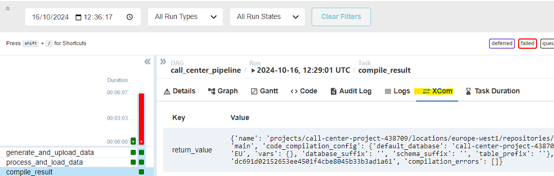
And we are done! The expected output is below:

You can now see your production table under sales_rep dataset:
SELECT * FROM call-center-project-438709.sales_rep.sales_rep_calls
Final step: Create Looker report
Now, directly from your table, you can create a Looker dashboard:

Congratulations! You’ve just built your first pipeline in GCP. If you want to run it daily, remember to change the schedule_interval to ‘@daily’!
Good luck in your future developments!